
For a downloadable version, click here.
Business intelligence, along with big data and analytics have emerged as three of the most important business trends of the twenty-first century. This has happened because of the convergence of:
- Connectivity – Everyone has ready access to data across networks, including modern techniques like restful interfaces.
- Computing power – Today, one can apply techniques, such as Monte Carlo simulation, on a laptop computer that not all that long ago required the use of mainframes.
- Availability of analytic tools – There is a range of laptop analytic tools available, including the very rich open-source analytics scripting language ‘R,’ inexpensive Monte Carlo tools, and Bayesian network tools.
The main reason for the trend is that analytics provides business owners and managers the insights they need to steer towards competitive advantage (e.g., Competing on Analytics by Thomas Davenport and Jeanne Harris). Analyzing the data has provided the means for businesses to be more agile in responding to their customers and to changing business situations.
Software has lagged in this trend. There are several barriers to adopting business intelligence in software development:
- There is no simple set of measures.
- Many organizations do not have or do not even know the data they need to support a useful measurement program.
- Analytic skills are not commonly found in in software development organizations.
Nevertheless, the same business pressures to adopt business intelligence and compete on analytics apply to software. It is now time for software organizations to adopt business intelligence techniques to get to the next level of agility.
‘Development intelligence’ is application of business intelligence to software and systems development.
In the following, a set of high-level principles are presented that should be considered when creating an analytics program. Then, there is a discussion of how to design an analytics solution for an organization, followed by a discussion of the different dimensions that must be considered when designing and building the solution.
The principles of software analytics
Agility requires control
In the early days of the Agile method of software development, some believed incorrectly that Agile was the rejection of disciplined software development. A better perspective is that Agile was a rejection of techniques, such as the waterfall lifecycle, that are ill-suited to the dynamics of software. In the early days, before Agile, project managers were told to ‘plan their work and work their plan.’ Thus, measurement systems, such as Earned Value Management (EVM), were designed to measure the extent of adherence to the plan.
Consider that agility is the ability to respond rapidly to the environment. A jet fighter is very agile, but it does not plan its route. Rather, it responds very rapidly to sudden changes in its environment, such as threats or its mission. It accomplishes this agility with very tight control loops, constantly measuring and reacting to its environment and its operation.
Agile software teams also must constantly respond to changes, such as:
- New or clarified requirements,
- Missed dependencies,
- Failed tests,
- Work taking longer than expected
This applies to software teams as well as to any level of the organization that relies on software development. Development organizations must respond to changing operational challenges, such as unpredictable team performance, disruptive technologies, labor arbitrage, and uncontrolled operations. In turn, the enterprise must respond to all of the above, along with evolving IT needs and/or market sentiment.
Control requires measures
It is not a new thought that measures are part of control loops. All responsive processes require some sort of control loop (Figure 1). Measures are central to the check step. These control loops are essential to any process that involves meeting goals.
If a team does not have a clear, ongoing view of its goals, its progress, and the likelihood of attaining its goals, it has no basis for reacting. Modern software analytics do not measure adherence to a plan; instead, thry provide the information that is needed to manage the control loops effectively and steer the team to success.

Figure 1. A control loop
Measures have cost
While control requires measures, they do not come without cost. First, significant manual effort may be required to collect the measures themselves, or some investment in automated data collection may be necessary. Even worse, collecting and driving the organization to the wrong analytics can lead to negative consequences. Such consequences can only be avoided by adopting analytics as part of a control loop that there is every intention of managing.
In brief,
“You can’t control what you don’t measure, and you shouldn’t measure what you don’t intend to manage.”
The right set of measures, chosen as part of the right control loop, promotes trust between the leadership and the staff. The wrong measures breed mistrust, waste time and resources, and drive undesired behavior. For example, some firms might measure the number of bugs removed. That measure might be part of the wrong control loop. That measure, along with productivity measures, could inadvertently reinforce sloppy coding. Improving quality takes a more subtle choice of measures.
Simple, but not too simple
Albert Einstein is often quoted as saying, “Everything should be made as simple as possible, but no simpler.” I call this the Einstein test. How this applies to measures is that the solution must be both consumable and correct. For measures to be consumable, they shouldn’t require a Ph.D. in statistics to understand. However, the sort of data generated by development organizations is far from simple, and simple measures, such as counts and averages, may be too simple to give the insight needed to take the right action. The right solution for your organization should be both simple and actionable.
Designing the measurement solution
For an organization to measure in a purposeful way, it must:
- Specify the goals for itself and its projects
- Trace the goals to the data that are required to track and confirm the attainment of the goals
- Provide a framework for interpreting the data with respect to the stated goals in order to take action.
The goal, question, metric (GQM) method is a design method for analytic solutions, much like noun-verb analysis in software design. It is a method to derive the metric’s solution from the organization’s goals.
Here is a summary of the steps in the GQM method:
- Specify a set of corporate, division, and project business goals and associated measurement goals.
- Specify a high-level model of the process and/or key artifacts identified in the goal; if necessary, decompose the qualitative goal to one or more quantitative goals.
- Generate questions based on the lifecycle model, for example: How would I know if improvement is attained? What are the measures of the business process (steps)? What do I need to know about the context to understand process execution, e.g., external sources of work?
- Study the data to specify the datasets, statistics, and analytics that must be collected to answer those questions and track progress toward achieving the goals.
- If the data are not available, specify the data that must be collected.
- Develop automated mechanisms for data collection and analytics.
- Collect, validate, and analyze the data to identify patterns that diagnose the operational situation with respect to the goal and possibly provide suggestions for corrective actions.
- Review the solution with stakeholders to make recommendations
Dimensions of software analytics
Choosing the right measure is not only crucial, it requires expertise. Analytics are multi-dimensional:
- Organization level
- What is measured
- Type of development
- Analytics Maturity
Each of the dimensions mentioned above are addressed below.
Organizational Level
As depicted in Figure 2, different levels of a development organization have different goals. For the organization to work for the enterprise, the goals at one level must support the goals of the level above. Generally, goals flow down the organization. Another perspective is that, for one level of the organization to meet its commitments, the lower levels must meet their commitments.
From above, different goals entail different control loops that, in turn, entail different analytics. However, one level’s operation depends on the operation of the lower levels. This is very reminiscent of ‘black box, white box’ reasoning in system architecture. At each level, the blackbox measures reflect the performance of the encapsulated level as seen from the outside. The white box measures are the internal measures of the level required to meet the black box measures.
Since a level depends on the lower level, it is essential that the lower level’s blackbox measures be fully visible to the upper level and that those measures support the upper level’s measures.
To summarize, a full measurement architecture must reflect that
- Different levels have different control loops and, thus, different measures
- Blackbox measures at one level become the whitebox measures at the upper level.
It follows that the architecture of the measures should reflect both the organizational architecture and the goal architecture.

Figure 2 Analytics vary with the organization level
What is measured
Organizations have a variety of goals. These can include better financial outcomes; faster time to market or, more generally, to value; operational efficiency, including adoption of lean principles and practices; and delivering higher quality. Of course, these goals are not independent. For example, a team could take advantage of the leaner operations to devote more attention to quality, which, in turn, could have a positive economic impact.
A measurement solution might consist of a mix of the following:
- Throughput/flow measures.
- These are based on product flow and queuing theory. They are useful in finding bottlenecks, eliminating waste, and streamlining operations.
- Project measures – Cost and schedule
- These measures track whether required or desired functionality is on track or likely to deliver on time and/or on budget. These include, but are not limited to, modern adaptations of earned value measures.
- Economic measures:
- In the end, software organizations’ goals are to deliver economic value to their stakeholders. Measuring that economic value can involve Net Present Value (NPV), Return on Investments (RoI), or Internal Rate of Return (IRR). These measures are often used in conjunction with portfolio management.
- Quality measures
- Another possible goal of an organization is to affordably improve the quality of its output to ‘good enough’ levels. However, measures of quality can range from simple defect counts to more complex measures, such as system reliability, after-market costs, and market sentiment.
- Practice adoption and adherence measures
- Some organizations’ goals are the adoption and execution of some set of practices. For example, these may be a set of Agile methods, DevOp methods, or something more domain-specific, such as testing practices.
While the adoption of practices may be a goal in itself, the practices are likely being adopted in order to achieve some other goal, such as reducing cycle time. One should adopt an analytics framework that measures both and perhaps adopt some predictive method, as discussed below, to show how one influences the other. Some use the terms ‘operational measures’ and ‘outcome measures’ to describe this pattern. In the example the practices are the operations, and the improvement of cycle time is the outcome.
Type of development
Software development falls roughly into three classes (Figure 3):
- Maintenance and small change requests
These activities involve making small changes to an existing code base. In most cases, they are applied to deployed code. The dynamics of this activity involve receiving and servicing an unsteady flow of problem reports or small enhancement requests. Typically such requests are detailed and well understood, and the team is able to estimate the time and effort required with high confidence. About 70% of what the industry spends is on these activities. These teams are increasingly adopting DevOps and continuous delivery practices.
- New features on existing platforms
These efforts are to add significant new features to an existing application. For example, a bank may have a mobile app for account holders. The business analysts decide that the app should add an online check deposit feature. This is a major undertaking that involves several teams and several months to accomplish. Once the team receives the feature request from the business analyst, it estimates the time and effort required. Unlike change requests, the team has less confidence in the estimates of time and effort, and it may run some experiments to learn what is needed to have more confidence in making commitments to deliver the feature to the business.
- New platform
Occasionally, a development organization gets the opportunity to build an entirely new application, a so-called greenfield project. This may be a small mobile app requiring the so-called one-pizza team building something on the cloud or a big integrated system requiring hundreds of developers or more. The project is initiated with some business need or idea but without detailed requirements or product design. Hence, the team has little basis for making estimates, and whatever estimates they make will be low confidence. Lean startup methods are especially useful for such efforts.

Figure 3. The three kinds of development.
Many organizations have a mix of these types of efforts.
The different sorts of development require different sorts of analytics. The maintenance and small change efforts have information that is suitable to descriptive statistics. The new platform teams have little data, but they may have prior beliefs based on expert opinion. This situation calls for predictive approaches. New feature development calls for a mixture of both.
Analytic Maturity
Software measurement techniques range from simple reports to deep, predictive analytics. The choice depends on the nature of the data and the question being answered by the analysis.
- Simple reports
- Descriptive statistics
- Predictive analytics
Each of these possible choices is described below.
Simple reports
These consist mostly of data counts, such as the number of defects that are currently open on a given date or perhaps the trend of averages. An example , the number of defects that are currently open on a given date is shown in Figure 3.

Figure 3. Example of a simple report
Descriptive Statistics
This is best explained with an example. Suppose the general goal of the organization is to reduce cycle time. Those responsible would start by exploring the population of the set of ages of currently open work items, and they would find that all of the open items have been open for different lengths of time. Some were opened recently, and some were opened some time ago. Figure 6 shows what a typical distribution of ages might look like. Notice that most of the items are just a few days old, but the tail is very long. This curve looks very little like the familiar bell-shaped curve shown in Figure 4. If the distribution looked like Figure 4, that would mean that the highest number (the mode) of the items took 25 days with an equal number taking more and less time.
Part of a good analytics program is to choose one or more statistics, i.e., a number that characterizes the distribution. For example, the usual choice for a center-weighted distribution is the mean ( average value) and standard deviation, a distance from the average that characterizes the width (Figure 5). Because the normal distribution is symmetrical, the mean is also the median, i.e., the 50% point. Half the values are above the average and half are below it. Further, about 68% of the data have values within one standard deviation. In the example, 64% of the items have an age between 19 and 31 days.

Figure 4. The common normal distribution, atypical for software data

Figure 5. Normal distributions with its mean and standard deviation
This raises the question concerning what statistic should be used for more realistic development data (Figure 6). One might choose the mean (15.3 days in Figure 7), but what does the mean tell us about the distribution? As you can see in Figure 8, the 50% point, the median, is significantly less, only 10.36 days. The mean is higher because it includes the age of old, stale items the ages of which may reflect poor backlog culling rather than the responsiveness of the team. So, with this sort of long-tailed distribution, the median or perhaps the 80% or 90% point would be a better measurement than the mean.

Figure 6. Typical distribution of the age of development items

Figure 7. The mean and standard deviation for a long-tailed distribution

Figure 8. Median and other percent points for a long-tailed distribution
These statistics are used for product flow measures to instantiate lean software, Kanban, and Don Reinertsen’s flow principles. These include, for example, lean times, cycle times, and backlog age.
Predictive Analytics
Going back to our control loop, once one has the information from the analytics to take action, there is still the problem of what actions to take. Before taking action, it would be good to know what is the probable outcome of the action. This is what is more generally called ‘what if’ analysis, a common use of spreadsheets.
Predictive analytics provide the means for describing what is the likely outcome of taking some action. As such, predictive analytics use the language of probability. A common predictive report is what is called a probability distribution (Figure 9).

Figure 9. Probability distribution
A probability distribution is much like a histogram, except that the total area under the curve is 1, representing the probability version of certainty. The vertical axis roughly corresponds to the probability of the event. The way to read a distribution is to treat the area under some region of the curve as the probability that one of those events will occur. For example, suppose the distribution represents when a project might ship. In this case, the events correspond to the days a product might ship, and, the higher the distribution, the more likely the product would ship on that day. In this case, we could determine, for example, that the probability of shipping between 10 and 20 is about 0.25 (Figure 10).

Figure 10. Area of the red zone is about 0.25
So, a predictive analytic returns a distribution that can be used to reason about the probability of events.
There is a variety of ways that a probability distribution can be computed. A powerful method uses what are called Bayesian nets, a technique based on Bayes theorem and conditional probability. These are built starting with a causal model of what is to be predicted. For example, suppose we want to predict the number of software defects that will be found in operation. Although we can’t predict with certainty, we might be able to find a distribution. We might build a causal network with Figure 11 that is shipped with the AgenaRisk tool. As can be seen from the model’s purple boxes, the number of defects found in the field depends on the complexity of the code, the quality of the design, and testing. Also, the more the code is used, the more likely defects will be found. These parameters can be used to determine the yellow boxes, i.e., the number of defects injected in the code and the number of defects discovered in testing. Other parameters could be added to the model, such as code size and coder quality.
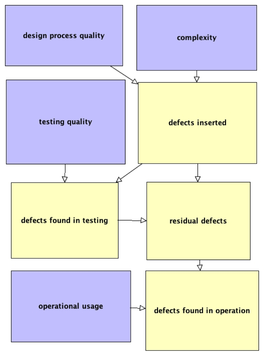
Figure 11. Model for predicting defects found in the field
Which box affects which is designated by the arrows. The expert who builds the model specifies the nature of that influence using appropriate probability models.
Such a model can be used to build different scenarios. For example, suppose that we assume the team has medium skills in building a complex code with high operational usage (Figure 12). The output of this model is the distribution in the lower right (Figure 13). It tells us that it is very probable that the number of defects found in operation will be somewhere between 10 and 30.

Figure 12. Scenario 1, business as usual

Figure 13. Distribution of predicted defects found in the operation in scenario 1
Now, further assume that the business determines that addressing this number of defects in operations is very costly, not only to repair but also to the reputation of the company, which would lead to lower revenue. It has been determined that this level of defects is costing the company about $20M/yr. So, there is an economic incentive to reduce the number of defects to no more than 5/yr. That is their goal. The question is, “What is the best path to take?” The company considers four scenarios.
- Business as usual – no change
- Invest heavily in testing improvement
- Invest in an improved process, leading to less complex designs
- Investing in both.
They use the model to test scenario 2 (Figure 14) and find, unsurprisingly, the outcome of improved testing shows much improvement (Figure 15). The distribution shows that, under this scenario, they are around 90% likely to have 10/yr or fewer defects in operation. The goal of fewer than 5/yr is an even bet.

Figure 14. Scnario 2

Figure 15. Distribution of predicted defects found in operation in scenario 2
Then, the team ran scenario 3 with the improved design process, resulting in a more elegant, less complex design. The result of the improved design (Figure 17) had less impact than scenario 2.

Figure 16. Scenario 3, better design

Figure 17. Distribution of predicted defects found in operation with the improved design
Finally, the team ran scenario 4 (Figure 18) with the desired outcome (Figure 19).

Figure 18. Scenario 4, improving both testing and design

Figure 19. Distribution of defects found in operation with both improved testing and design
Table 1 provides a summary of the results.
| Scenario | Action | Median No. of defects | 75% defects |
| 1 | Business as usual | 18 | 24 |
| 2 | Invest in testing | 3 | 6.3 |
| 3 | Invest in design | 6 | 10.4 |
| 4 | Both | 1 | 2.6 |
Table 1
The way to read the table is that there is a better than even chance that investing in testing will meet the goal, but it is not certain. In fact, there is a 25% chance that there will be more than six defects. The only way to be close to certain that the goal will be met is to invest in both.
In the end, the business is faced with an economic decision. The scenario that should be implemented depends on the cost to the business and ultimately its return on investment (ROI) in terms of the savings in operational expense and avoidance of lost revenue over the costs of the improvements. This ROI involves uncertain quantities, so the use of predictive methods is required. It can be determined in a reasonably straightforward way using Monte Carlo simulation tools.
Summary: What conversation do you need to have?
Some fear that building an analytic solution somehow takes the human element out of the process. That is far from the truth. Analytics provide information that empowers people to make decisions and take action. Ideally, this is best done with concurrence across the levels of an organization. A good program manager takes actions that make sense to his staff and that can be explained to his managers. The same concept works for senior managers and even C-level executives. In each case, taking action entails people discussing what the best courses of action are.
Without analytics, people will often make assertions and state opinions with or without foundations. Often the most assertive or insistent person determines the outcome. With analytics, the participants can have a reasoned discussion based on evidence and its implications. A mentor of mine often said,“In God we trust, everyone else brings data.” Perhaps he should have said, “… everyone else provides the analytics.”